This protocol describes a static compression test for evaluating the mechanical properties of 3D-printed scaffolds. Static compression test can be performed for 3D bioprinted hydrogel-based scaffolds using TA instruments. To mimic the physiological environment of the body, it is recommended to perform the compression test in a wet condition at 37 °C. Wet scaffolds should be soaked in PBS previously for 24-48 hours. The dry scaffolds could also be tested as a control. The steps of the protocol are listed below.
- Parallel plates and a suitable geometry of HR-20 Rheometer (TA Instruments, New Castle, DE, USA) should be selected.
- Put the scaffolds in the center of the plate and cut the scaffolds into the same size according to the shape and diameter of the upper geometry. For wet samples, PBS needs to be added to the bottom plate around the scaffold.
- Adjust the height of your scaffold using a Vernier caliper. This could be considered the initial gap.
- Adjust the upper geometry to contact the surface of the scaffold without applying forces (initial force 0 N axial force). This could be done manually or by inserting the value of the gap, which was measured in the third step in the Triose software (Please pay attention not to squeeze your sample in this step).
- The compression test was initiated using TRIOS software at a constant speed (e.g., 1 µm/s). Following this step, the machine starts compression until it reaches the highest pressure, which is 50 N.
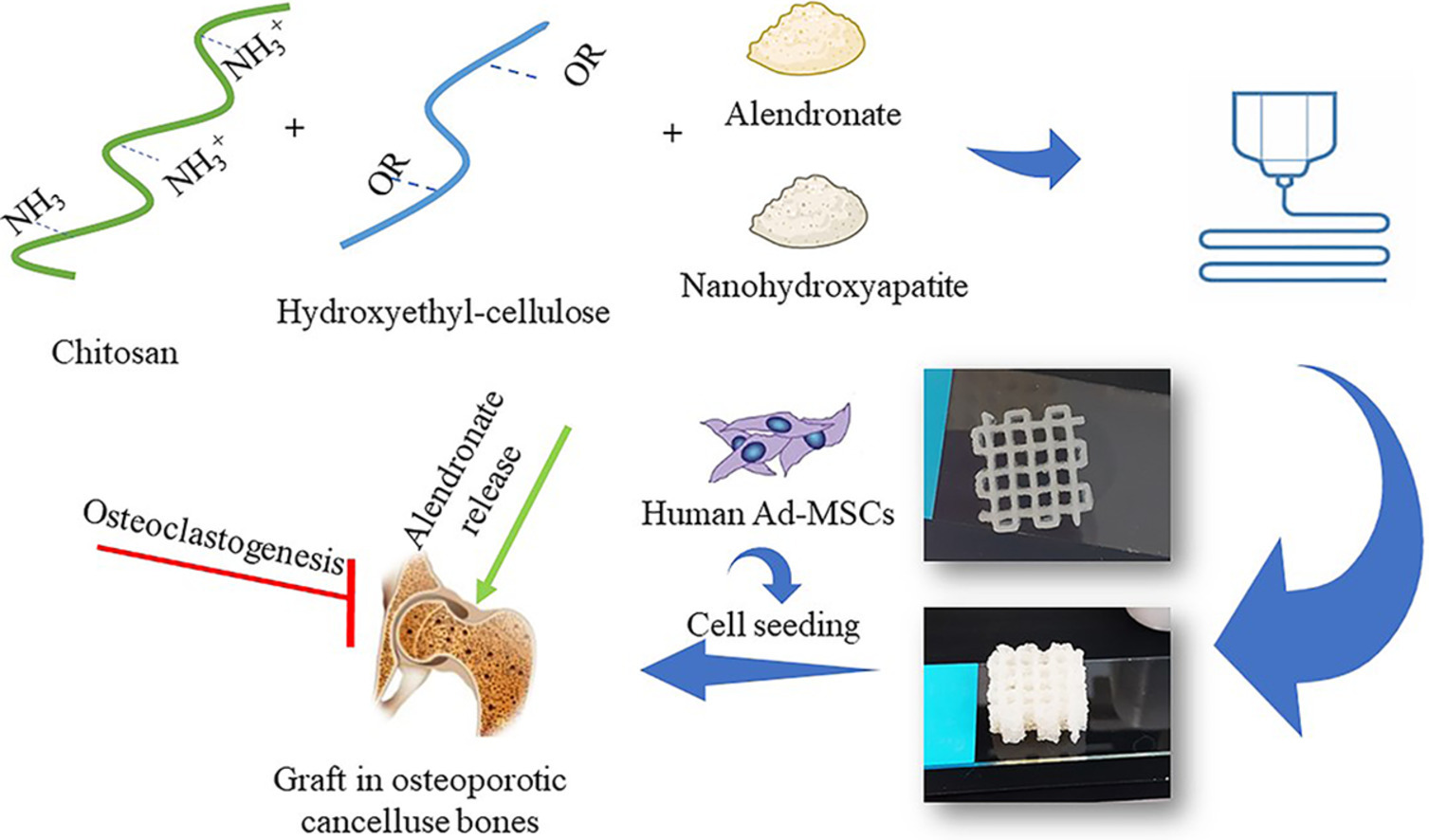
- The first graph that the machine provides you is an axial force versus step time graph (Figure 1). Following the blue line, which represents the axial force, it shows that the force started from 0N and increased to reach a peak of 50N, then fell to reach a plateau phase. The graph shows, while the axial force is rising, the initial gap is decreasing. This behaviour of hydrogels is predictable. As you can see in Figure 1, the test was performed in duplicate, and the results showed good reproducibility.
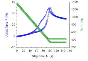
Figur1. Compression test with repeats. Axial test versus gap. - To calculate the compressive modulus, you need to change the axial force on X axis to stress and the Y axis to Strain value. The slope of the first linear phase is your compressive modulus. You can interpret your graph in the other way additionally. At the same strain, the sample, which stands higher stress, is stiffer, and its compressive modulus is higher (Figure 2). You can use Prism GraphPad for statistical analysis of your compressive modulus among your samples. To find the first most linear phase of the graph, you need to export the data up to 20% strain to an Excel file to detect better, and then the most linear phase is approximately up to 5% (Figure 3). Compressive modulus values were extracted from the slope of the first linear region (usually 0–5% strain).
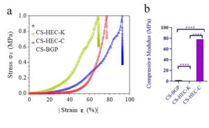
Figure 2. Compressive stress-stain curves. compressive modulus of CS-BGP, CS-HEC-K and CS-HEC-C (Name of different samples). ANOVA with Tukey’s multiple comparisons tests; ****p < 0.0001. 
Figure 3. Linear region used for modulus calculation.
References:
- Afra, S., Koch, M., Żur-Pińska, J., Dolatshahi, M., Bahrami, A. R., Sayed, J. E., Moradi, A., Matin, M. M. & Włodarczyk-Biegun, M. K. (2024). Chitosan/Nanohydroxyapatite/Hydroxyethyl-cellulose-based printable formulations for local alendronate drug delivery in osteoporosis treatment. Carbohydrate Polymer Technologies and Applications 7: 100418.
| Number | Category | Product | Amount |
|---|
5 thoughts on “Protocol for static compression testing of printed hydrogel scaffolds”